
In July 2023, Kenya faced a potato shortage, leaving harvest off-takers scrambling to find potato suppliers. Although the off-takers know in which parts of the country potatoes can generally be found, they still had to deal with a vast area where they needed to locate potato fields.
At agriBORA, we’ve been working closely with different off-takers and listening to their challenges. In this article, we’ll explain how we tackled these challenges with advanced crop type mapping techniques. Especially we focus on Uasin Gishu county, which is one of the main potato growing counties. The aim of our analysis is to produce a map at the field level, that indicates in which fields potatoes are grown.
Explore the data
Our approach starts with a dataset of 1250 fields in Uasin Gishu, Kenya, which includes information about the crops planted in 2023. This dataset has a major imbalance, because most fields are planted with maize, the most common crop in Uasin Gishu County.
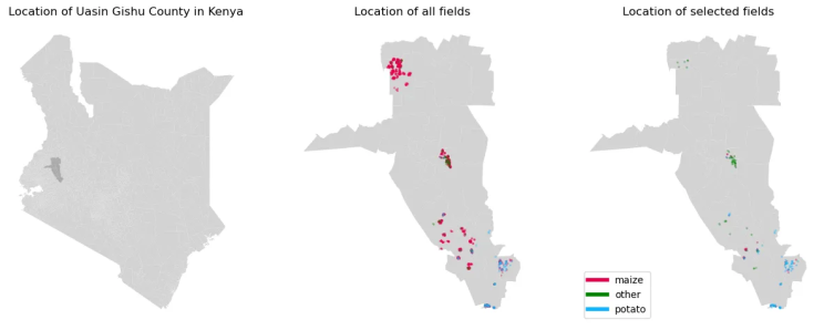
We furthermore face the challenge, that the mapped crop types are not evenly distributed throughout the county. As we can see in the map, fields with potato production were mostly registered in the south, whereas there is a larger cluster of maize fields recorded in the north of the county. However we do not want the model to learn to detect whether a field is in the north or south of the county, but to differentiate potato fields from other fields. To improve the dataset’s balance and spatial diversity, we did the following:
- Potato Fields: We selected all 103 fields where potatoes were grown, as this is the entity we are most interested in.
- Maize Fields: To make the dataset fairer, we chose 52 maize fields to ensure maize was not overrepresented in the dataset. In order to account for the spatial distribution, we only selected maize fields, that were located within a short distance from potato fields.
- Fields with other crops: We included all 55 fields categorized as “other,” adding variety to our dataset to account for different crop types.
By doing this, we’ve created a more balanced dataset. This dataset forms the basis of our solution, helping us pinpoint potato fields more accurately and assisting offtakers in their search for reliable potato suppliers.
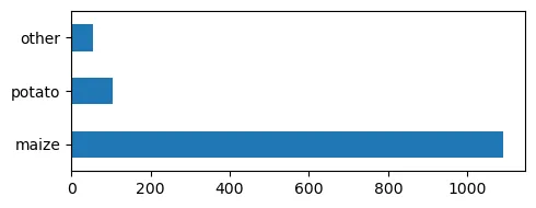

Original number of fields per croptype.
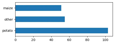

Number of fields per crop type in the final dataset.
Retrieve Sentinel Images
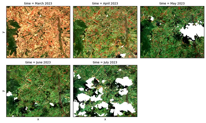
We are looking at the crops planted during the long rain season (LRS) of 2023, which ranges roughly from March to end of July. For this period we downloaded the Sentinel-2 L2A product. The processing included:
- cloud masking: here we are using the s2cloudless algorithm.
- calculating vegetation indices: - CVI: Chlorophyll vegetation index (B08∗B04)/(B03)² - PPR: Plant pigment ratio (B03-B02)/(B03+B02)
- resample the data to monthly resolution
Train the model
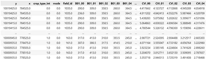
For our crop type map we use the random forest implementation of sklearn. Therefore we first needed to transform the Sentinel 2 images into a data format, that is readable by sklearn. The resulting dataframe has one column for each predictor at every timestep.
Now we can build our model. Here we opted for a simple hyperparameter tuning approach, where we looked at the parameters n_estimators and max_depth. A validation accuracy of 0.906 was achieved using n_estimators = 30 and max_depth = 20.
from sklearn.ensemble import RandomForestClassifier
n_estimators = [10, 20, 30]
max_depths = [None, 20, 30]
scores = []
for n_estimator in n_estimators:
for max_depth in max_depths:
model = RandomForestClassifier(n_estimators=n_estimator,
max_depth = max_depth,
random_state=42,
max_features = "sqrt",
class_weight = "balanced")
model.fit(df2.loc[df2["mode"] == 0, predictors],
df2.loc[df2["mode"] == 0, target].astype("int8"))
scores.append(model.score(df2.loc[df2["mode"] == 1, predictors],
df2.loc[df2["mode"] == 1, target]))
combined = []
for pair in itertools.product(*[n_estimators, max_depths]):
combined.append(pair)
print(f"best score ({np.round(np.max(scores), 3)}) was achieved with n_estimators = {combined[np.argmax(scores)][0]} and max_depth = {combined[np.argmax(scores)][1]}.")
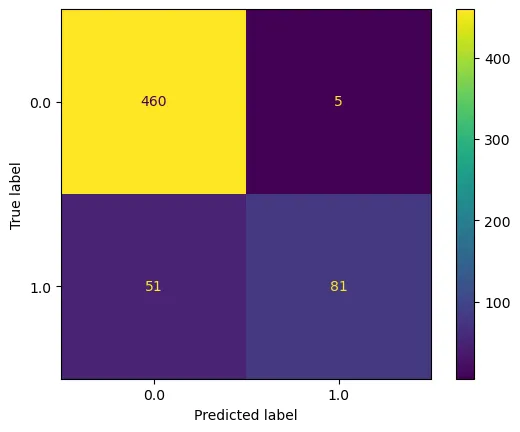
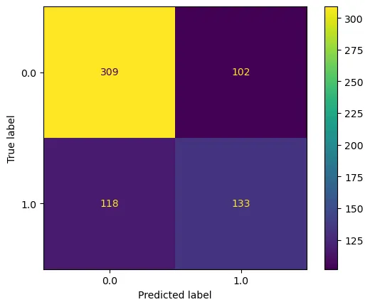
# best score (0.906) was achieved with n_estimators = 30 and max_depth = 20.We should note, that the accuracy score might be misleading here, since the accuracy is very sensitive to class imbalances. In the confusion matrix below, we can see, that
- there are a lot more 0 instances than 1 in the validation dataset. This is because we didn’t check for field sizes when splitting the dataset into train / validation / test. Apparently the non-potato fields were on average larger than the potato fields.
- from the 132 potato datapoints, 51 were predicted as non-potatos, which is very poor outcome. The model is quite conservative in predicting potatoes.
The final model achieved an accuracy of 0.668 on the test data set, which is a large drop compared to the validation score. This indicates that we overfitted our model.
How could we improve this result?
- Of course more and better data is always a good idea. Especially a more diverse data set, both concerning crop types and field locations, could improve the results.
- Build the training data set more carefully, for example by taking into account the size of the fields.
- Implement a more elaborated hyper parameter tuning using cross validation and more parameters.
Predict distribution of potatoes
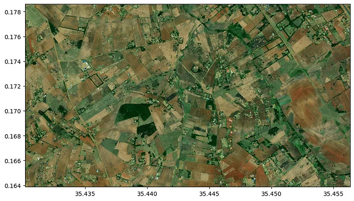
For now, let’s go on with our mediocre model and predict the occurance of fields planted with potatoes. We therefore selected a small area in Uasin Gishu. For the purpose of better visualization we show the 0.5 m resolution ESRI basemap image. The crop type mapping is of course done using the Sentinel-2 data.
Create Crop Map
Since the crop type model was only trained on agricultural fields, it cannot differentiate between crop land and other landuse types. Therefore, we first define a simple cropland classifier, which is based on the range of the NDVI during the season. The intuition here is, that the amount of vegetation that is present at an agricultural field shows a higher variation during the season compared to other land use types.
# calculate NDVI
s2_data["NDVI"] = (s2_data["B08"] - s2_data["B04"]) /
                  (s2_data["B08"] + s2_data["B04"])

# calculate NDVI range
NDVI_quantiles = s2_data["NDVI"].quantile((0.05, 0.95), "time")

ndvi_range = NDVI_quantiles.sel(quantile = 0.95) -
              NDVI_quantiles.sel(quantile = 0.05)

# define crop mask, where values > 0.35 are crops
crop_mask = ndvi_range > 0.35
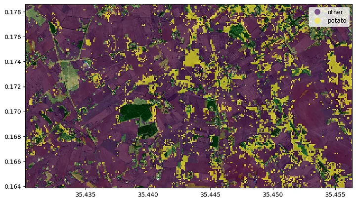
Create Crop Type Map
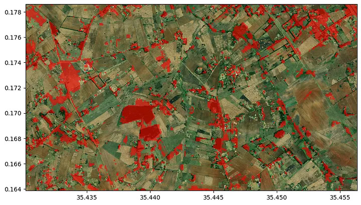
Now we can go on and predict the distribution of potato fields in the area. The prediction is then masked with the crop mask. We can see that most of the area is planted with other crops, than potatoes (most likely maize).
Get Crop prediction at field level
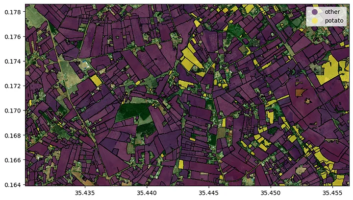
To get a better impression of the agricultural landscape, we can apply our field delineation model in order to get field outlines. This model was trained using high resolution satellite imagery. If you want to know more about the field delineation algorithm please refer to the paper published by Waldner et al. (2021), the follow-up paper by Wang et al. (2022) or this medium article.
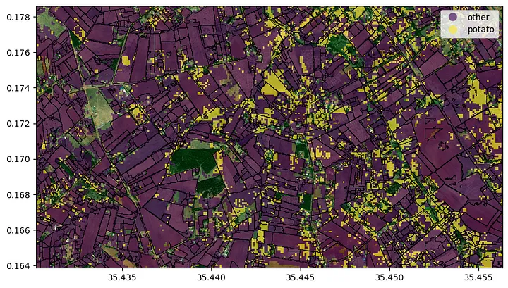
In the image above, we simply overlaid the crop type prediction with the field outlines. Now we can do a simple majority voting to assign the crop types to the fields and voilà, here is our map of potato fields for the off takers.
About agriBORA
agriBORA is a Kenyan-German agri-Fin-Tech platform that has developed a B2B2C Software as a Service solution to empower local agribusinesses with digital tools and processes that can improve farm productivity and facilitate effective trading between them and farmers. The agriBORA technology combines basic feature phone functionalities such as SMS, USSD and mobile payment solutions with advanced analytics based on Earth observation satellite data to monitor and assess crop development during the season. Visit the agriBORA website here at https://agribora.com to learn more about our work.
About the author
Lena Perzlmaier is a Data Scientist at agriBORA, specializing in Earth Observation. She analyzes remote sensing data for agricultural use cases in Eastern Africa. Her main areas of expertise are crop type mapping, field delineation and field NDVI trends analysis.